Business Calculus
Business Calculus
Business Calculus Formulating Business Data
1.The three processes of business calculus
The three processes of business calculus are: Obtaining business data, formulating data and making business decisions through calculus. The first process acquires and prepares various business data such as sales, expenses, man-hours, cashflows, assets, liabilities, and investment projects. The second process is to formulate these business data so that they can be processed with calculus. This process relies heavily on various analysis methods and Excel. If we can formulate it, we will process it with calculus in the third process and make a business decision. Formulating business data is the most error-prone of the three processes, and it is often difficult in practice. In business calculus, it can be said that the ability to express concepts in mathematical formulas is a key success factor.
As preparation for analysis, data analysis (single regression, multiple regression) and solver must be added to Excel. Click on the data tab in Excel and check whether "Solver" and "Data Analysis" are displayed on the right side respectively. If it is not displayed, please add-in.
2.Simple Regression Analysis
In calculus, we use techniques such as simple regression analysis, multiple regression analysis and least squares method. These methods involve the formulation of a mathematical equation, y = f(x), when y is a continuous variable, based on the data x. In other words, it involves fitting a model between a dependent variable (y) and one or more independent variables (x) on a continuous scale. When there is only one x variable, it is called simple regression, and when there are multiple x variables, it is called multiple regression. The most basic model used in regression analysis is linear regression in the form of y = Ax + B.
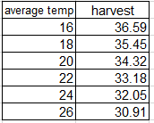
Check out the Excel regression analysis method in the following example where the harvest of a certain fruit (y is the dependent variable) depends on the mean temperature (x is the independent variable).
[Example] Effect of average temperature on harvest.
Data-> Data analysis -> Regression analysis -> Input Y(Q), Input X(P)-> OK
Input Y Range : Dependency change number (wrap labeled column)
Input X Range : Independent variable (wrap the label column)
Label: If checked at the time of output, it becomes the label (average temp)
Output options : Output Range
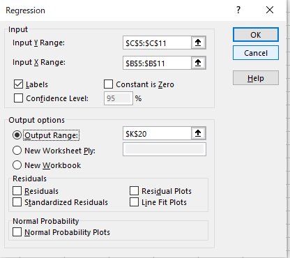
Results are displayed
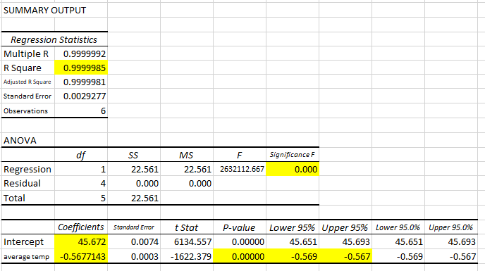
1)Regression formula y = 45.672-0.567714x <-The business data has been formulated!
2)Coefficient of determination R2: The closer the value is to 1, the higher the analytical accuracy.
R2= 0.9999985 with very high analysis accuracy = = > OK
R2= R^2 (squared multiplication of correlation coefficient R)
Correction R2: Correction because it becomes larger as the number of explanatory variables increases
3)P-value(significance probability): Statistically significant if less than 0.05 Significant
for all less than 0.05 ==>OK
4)Lower limit 95% / Upper limit 95%: If data is taken 100 times, about 95times are within this range
All within the range ==> OK
3.Multiple Regression Analysis
Multiple regression analysis, as mentioned above, refers to cases where there are two or more independent variables (explanatory variables) x. In the following example, we have three independent variables: maximum temperature, maximum humidity, and maximum wind speed.
[Example]
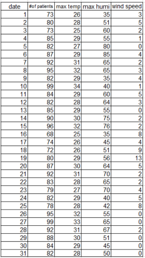
The number of patients who were transported by ambulance due to heatstroke in July in A city, and the maximum temperature, maximum humidity, and maximum wind speed of the day are as follows.
Predict the number of patients on a day with maximum temperature = 35C, maximum humidity = 50%, and maximum wind speed = 0
1)Implementation of multiple regression analysis.
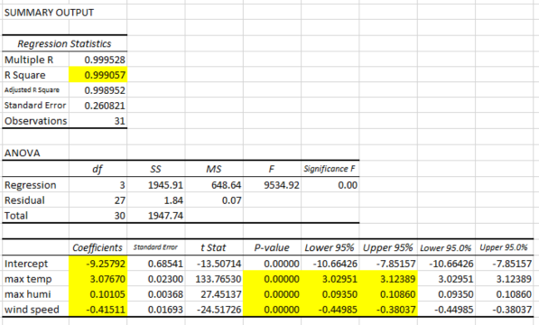
2)Evaluation of multiple regression analysis.
(1) Regression formula: number of patients = -9.257 +3.076 x temperature + 0.101 x humidity - 0.415 x wind speed
<-The business data has been formulated! The higher the temperature and humidity, the higher the number of patients, and the higher the wind, the lower the number.
(2) Coefficient of determination R2: The closer to 1, the higher the analytical accuracy
R2 = 0.999057, which is very high analysis accuracy ==> OK
(3) P value (significance probability): Statistically significant when less than 0.05.
All less than 0.05 ==>OK
(4) Lower limit 95%/Upper limit 95%: If data is taken 100 times, about 95 times are within this range.
3)Predicted number of patients on a day with maximum temperature = 35C, maximum humidity = 50%, and maximum wind speed =0
Number of patients=-9.257 + 3.076*35 + 0.101*50-0.415*0
= 103.453 -> 103predicted The number of patients is 103.
4.Least Squares Method
The method of least squares is a way to determine the coefficients of a presumed function, such as a linear function or a logarithmic curve, that provides a good approximation to a set of business data points. It involves minimizing the sum of squared residuals, ensuring that the assumed function is a close fit to the measured values. This technique can be analyzed using tools like Excel Solver.
[Example]
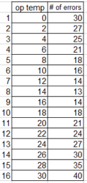
The following shows the number of error occurrences for the hot-selling product Z of the precision machinery manufacturer A, depending on the operating temperature. Find an approximation formula.

[Answer]
Imagine a graph and solve the quadratic polynomial (y=ax^2+bx+c).
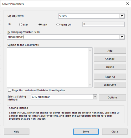
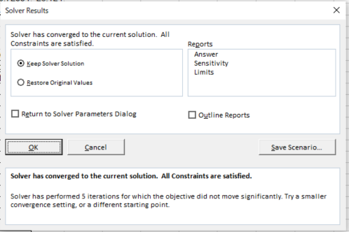
Solver Parameters
*Set Objective: total of (f(x)−Y)^2 *To: Min *By Changing Variable Cells: a,b,c
*Uncheck to make the number of limits of a, b, c, d non-negative
*Keep Solver Solution -> OK
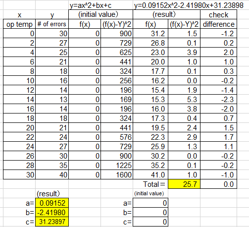
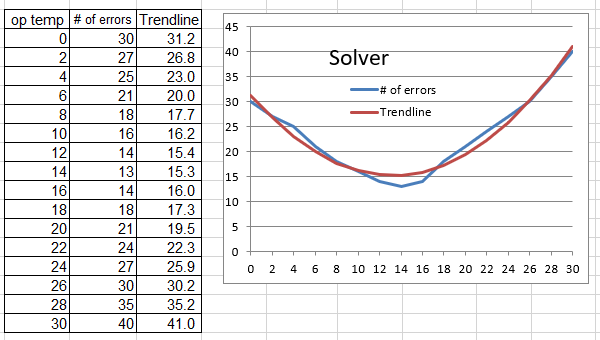
y=0.09152x^2-2.41980x+31.238987 <-The business data has been formulated!
5.Excel Approximation Curve
In addition to regression analysis and the method of least squares, Excel has a convenient function called approximate curve that is very useful in business calculus. The method for selecting each trendline is as follows. Polynomial and linear approximations are frequently used in business calculus.
*Polynomial approximation : The shape of the graph increases or decreases
*Linear approximation : Increases or decreases, but the way of change does not change(linear)
*Exponential approximation or power approximation : Increases or decreases, but the way of change becomes larger
*Logarithmic approximation : increases or decreases and the way of change becomes smaller and does not converge
*Moving average: increases or decreases and the way of change becomes smaller and converges
In the following example, the approximate curve by Excel. Please check how to find.
[Example]
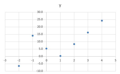
Find the approximate formula for the following data.
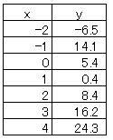
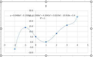
Since y is increasing and decreasing, we will use polynomial approximation. Just in case, let's find the approximation formulas from the 4th to the 6th order.
Insert -> Scatterplot -> Select scatterplot (upper left) -> Select data -> Range of graph data(C4:D11) Select XY -> OK
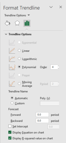
Layout ->Trendline
Other trendline options such as linear trendline

Polynomial Approximation Order can be selected from 2 to 6 ->Close
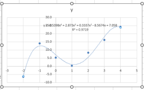
The formula and R2 value can be displayed on the graph
*Check the box to display the Equation on chart
*Check the box to display the R-squared value on the graph
Order = 4: R2 = 0.9719 and a small error with the 4th order
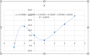
Order = 5: R2 = 0.9979 with a small error with the 5th order
Order = 6: R2 = 1 is OK Perfect with the 6th order
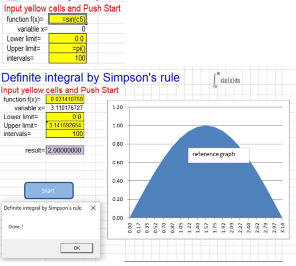
6.Integral by Simpson's rule (Integral Calculator)
In practical business calculus, the definite integral by Simpson's rule of is often used as a standard tool. Complex definite quantiles can be calculated simply and quickly. This program is written by N.Ishinabe using in VBA, so the macros should be enabled. Easy to use, just "Input yellow cells and Push Start".
Download from here Simpson's rule
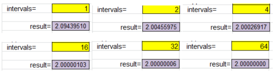
[Example 1] The calculation should result in 2.0.
intervals reflect accuracy ...
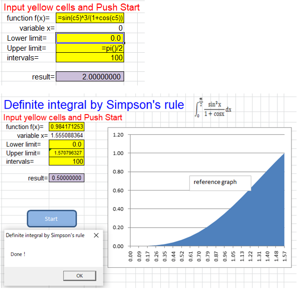
[Example2] The calculation should result in 0.5
A quick note on business calculus :Definite integral value from 0 to 1: AB ration is proportional to the order of y=x^n